Getting started with the Keras Sequential model

The Sequential model is a linear stack of layers.

You can create a Sequential model by passing a list of layer instances to the constructor:

from keras.models import Sequential
from keras.layers import Dense, Activation

model = Sequential([
    Dense(32, input_dim=784),
    Activation('relu'),
    Dense(10),
    Activation('softmax'),
])

You can also simply add layers via the .add() method:

model = Sequential()
model.add(Dense(32, input_dim=784))
model.add(Activation('relu'))

---

Specifying the input shape

The model needs to know what input shape it should expect. For this reason, the first layer in a Sequential model (and only the first, because following layers can do automatic shape inference) needs to receive information about its input shape. There are several possible ways to do this:

• pass an input_shape argument to the first layer. This is a shape tuple (a tuple of integers or None entries, where None indicates that any positive integer may be expected). In input_shape, the batch dimension is not included.
• pass instead a batch_input_shape argument, where the batch dimension is included. This is useful for specifying a fixed batch size (e.g. with stateful RNNs).
• some 2D layers, such as Dense, support the specification of their input shape via the argument input_dim, and some 3D temporal layers support the arguments input_dim and input_length.

As such, the following three snippets are strictly equivalent:

model = Sequential()
model.add(Dense(32, input_shape=(784,)))

model = Sequential()
model.add(Dense(32, batch_input_shape=(None, 784)))
# note that batch dimension is "None" here,
# so the model will be able to process batches of any size.

model = Sequential()
model.add(Dense(32, input_dim=784))

And so are the following three snippets:

model = Sequential()
model.add(LSTM(32, input_shape=(10, 64)))

model = Sequential()
model.add(LSTM(32, batch_input_shape=(None, 10, 64)))

model = Sequential()
model.add(LSTM(32, input_length=10, input_dim=64))

---

The Merge layer

Multiple Sequential instances can be merged into a single output via a Merge layer. The output is a layer that can be added as first layer in a new Sequential model. For instance, here's a model with two separate input branches getting merged:

from keras.layers import Merge

left_branch = Sequential()
left_branch.add(Dense(32, input_dim=784))

right_branch = Sequential()
right_branch.add(Dense(32, input_dim=784))

merged = Merge([left_branch, right_branch], mode='concat')

final_model = Sequential()
final_model.add(merged)
final_model.add(Dense(10, activation='softmax'))

Such a two-branch model can then be trained via e.g.:

final_model.compile(optimizer='rmsprop', loss='categorical_crossentropy')
final_model.fit([input_data_1, input_data_2], targets)  # we pass one data array per model input

The Merge layer supports a number of pre-defined modes:

• sum (default): element-wise sum
• concat: tensor concatenation. You can specify the concatenation axis via the argument concat_axis.
• mul: element-wise multiplication
• ave: tensor average
• dot: dot product. You can specify which axes to reduce along via the argument dot_axes.
• cos: cosine proximity between vectors in 2D tensors.

You can also pass a function as the mode argument, allowing for arbitrary transformations:

merged = Merge([left_branch, right_branch], mode=lambda x, y: x - y)

Now you know enough to be able to define almost any model with Keras. For complex models that cannot be expressed via Sequential and Merge, you can use the functional API.

---

Compilation

Before training a model, you need to configure the learning process, which is done via the compile method. It receives three arguments:

• an optimizer. This could be the string identifier of an existing optimizer (such as rmsprop or adagrad), or an instance of the Optimizer class. See: optimizers.
• a loss function. This is the objective that the model will try to minimize. It can be the string identifier of an existing loss function (such as categorical_crossentropy or mse), or it can be an objective function. See: objectives.
• a list of metrics. For any classification problem you will want to set this to metrics=['accuracy']. A metric could be the string identifier of an existing metric (only accuracy is supported at this point), or a custom metric function.

# for a multi-class classification problem
model.compile(optimizer='rmsprop',
              loss='categorical_crossentropy',
              metrics=['accuracy'])

# for a binary classification problem
model.compile(optimizer='rmsprop',
              loss='binary_crossentropy',
              metrics=['accuracy'])

# for a mean squared error regression problem
model.compile(optimizer='rmsprop',
              loss='mse')

---

Training

Keras models are trained on Numpy arrays of input data and labels. For training a model, you will typically use the fit function. Read its documentation here.

# for a single-input model with 2 classes (binary):

model = Sequential()
model.add(Dense(1, input_dim=784, activation='softmax'))
model.compile(optimizer='rmsprop',
              loss='binary_crossentropy',
              metrics=['accuracy'])

# generate dummy data
import numpy as np
data = np.random.random((1000, 784))
labels = np.random.randint(2, size=(1000, 1))

# train the model, iterating on the data in batches
# of 32 samples
model.fit(data, labels, nb_epoch=10, batch_size=32)

# for a multi-input model with 10 classes:

left_branch = Sequential()
left_branch.add(Dense(32, input_dim=784))

right_branch = Sequential()
right_branch.add(Dense(32, input_dim=784))

merged = Merge([left_branch, right_branch], mode='concat')

model = Sequential()
model.add(merged)
model.add(Dense(10, activation='softmax'))

model.compile(optimizer='rmsprop',
              loss='categorical_crossentropy',
              metrics=['accuracy'])

# generate dummy data
import numpy as np
from keras.utils.np_utils import to_categorical
data_1 = np.random.random((1000, 784))
data_2 = np.random.random((1000, 784))

# these are integers between 0 and 9
labels = np.random.randint(10, size=(1000, 1))
# we convert the labels to a binary matrix of size (1000, 10)
# for use with categorical_crossentropy
labels = to_categorical(labels, 10)

# train the model
# note that we are passing a list of Numpy arrays as training data
# since the model has 2 inputs
model.fit([data_1, data_2], labels, nb_epoch=10, batch_size=32)

---

Examples

Here are a few examples to get you started!

In the examples folder, you will also find example models for real datasets:

• CIFAR10 small images classification: Convolutional Neural Network (CNN) with realtime data augmentation
• IMDB movie review sentiment classification: LSTM over sequences of words
• Reuters newswires topic classification: Multilayer Perceptron (MLP)
• MNIST handwritten digits classification: MLP & CNN
• Character-level text generation with LSTM

...and more.

Multilayer Perceptron (MLP) for multi-class softmax classification:

from keras.models import Sequential
from keras.layers import Dense, Dropout, Activation
from keras.optimizers import SGD

model = Sequential()
# Dense(64) is a fully-connected layer with 64 hidden units.
# in the first layer, you must specify the expected input data shape:
# here, 20-dimensional vectors.
model.add(Dense(64, input_dim=20, init='uniform'))
model.add(Activation('tanh'))
model.add(Dropout(0.5))
model.add(Dense(64, init='uniform'))
model.add(Activation('tanh'))
model.add(Dropout(0.5))
model.add(Dense(10, init='uniform'))
model.add(Activation('softmax'))

sgd = SGD(lr=0.1, decay=1e-6, momentum=0.9, nesterov=True)
model.compile(loss='categorical_crossentropy',
              optimizer=sgd,
              metrics=['accuracy'])

model.fit(X_train, y_train,
          nb_epoch=20,
          batch_size=16)
score = model.evaluate(X_test, y_test, batch_size=16)

Alternative implementation of a similar MLP:

model = Sequential()
model.add(Dense(64, input_dim=20, activation='relu'))
model.add(Dropout(0.5))
model.add(Dense(64, activation='relu'))
model.add(Dropout(0.5))
model.add(Dense(10, activation='softmax'))

model.compile(loss='categorical_crossentropy',
              optimizer='adadelta',
              metrics=['accuracy'])

MLP for binary classification:

model = Sequential()
model.add(Dense(64, input_dim=20, init='uniform', activation='relu'))
model.add(Dropout(0.5))
model.add(Dense(64, activation='relu'))
model.add(Dropout(0.5))
model.add(Dense(1, activation='sigmoid'))

model.compile(loss='binary_crossentropy',
              optimizer='rmsprop',
              metrics=['accuracy'])

VGG-like convnet:

from keras.models import Sequential
from keras.layers import Dense, Dropout, Activation, Flatten
from keras.layers import Convolution2D, MaxPooling2D
from keras.optimizers import SGD

model = Sequential()
# input: 100x100 images with 3 channels -> (3, 100, 100) tensors.
# this applies 32 convolution filters of size 3x3 each.
model.add(Convolution2D(32, 3, 3, border_mode='valid', input_shape=(3, 100, 100)))
model.add(Activation('relu'))
model.add(Convolution2D(32, 3, 3))
model.add(Activation('relu'))
model.add(MaxPooling2D(pool_size=(2, 2)))
model.add(Dropout(0.25))

model.add(Convolution2D(64, 3, 3, border_mode='valid'))
model.add(Activation('relu'))
model.add(Convolution2D(64, 3, 3))
model.add(Activation('relu'))
model.add(MaxPooling2D(pool_size=(2, 2)))
model.add(Dropout(0.25))

model.add(Flatten())
# Note: Keras does automatic shape inference.
model.add(Dense(256))
model.add(Activation('relu'))
model.add(Dropout(0.5))

model.add(Dense(10))
model.add(Activation('softmax'))

sgd = SGD(lr=0.1, decay=1e-6, momentum=0.9, nesterov=True)
model.compile(loss='categorical_crossentropy', optimizer=sgd)

model.fit(X_train, Y_train, batch_size=32, nb_epoch=1)

Sequence classification with LSTM:

from keras.models import Sequential
from keras.layers import Dense, Dropout, Activation
from keras.layers import Embedding
from keras.layers import LSTM

model = Sequential()
model.add(Embedding(max_features, 256, input_length=maxlen))
model.add(LSTM(output_dim=128, activation='sigmoid', inner_activation='hard_sigmoid'))
model.add(Dropout(0.5))
model.add(Dense(1))
model.add(Activation('sigmoid'))

model.compile(loss='binary_crossentropy',
              optimizer='rmsprop',
              metrics=['accuracy'])

model.fit(X_train, Y_train, batch_size=16, nb_epoch=10)
score = model.evaluate(X_test, Y_test, batch_size=16)

Architecture for learning image captions with a convnet and a Gated Recurrent Unit:

(word-level embedding, caption of maximum length 16 words).

Note that getting this to work well will require using a bigger convnet, initialized with pre-trained weights.

max_caption_len = 16
vocab_size = 10000

# first, let's define an image model that
# will encode pictures into 128-dimensional vectors.
# it should be initialized with pre-trained weights.
image_model = Sequential()
image_model.add(Convolution2D(32, 3, 3, border_mode='valid', input_shape=(3, 100, 100)))
image_model.add(Activation('relu'))
image_model.add(Convolution2D(32, 3, 3))
image_model.add(Activation('relu'))
image_model.add(MaxPooling2D(pool_size=(2, 2)))

image_model.add(Convolution2D(64, 3, 3, border_mode='valid'))
image_model.add(Activation('relu'))
image_model.add(Convolution2D(64, 3, 3))
image_model.add(Activation('relu'))
image_model.add(MaxPooling2D(pool_size=(2, 2)))

image_model.add(Flatten())
image_model.add(Dense(128))

# let's load the weights from a save file.
image_model.load_weights('weight_file.h5')

# next, let's define a RNN model that encodes sequences of words
# into sequences of 128-dimensional word vectors.
language_model = Sequential()
language_model.add(Embedding(vocab_size, 256, input_length=max_caption_len))
language_model.add(GRU(output_dim=128, return_sequences=True))
language_model.add(TimeDistributed(Dense(128)))

# let's repeat the image vector to turn it into a sequence.
image_model.add(RepeatVector(max_caption_len))

# the output of both models will be tensors of shape (samples, max_caption_len, 128).
# let's concatenate these 2 vector sequences.
model = Sequential()
model.add(Merge([image_model, language_model], mode='concat', concat_axis=-1))
# let's encode this vector sequence into a single vector
model.add(GRU(256, return_sequences=False))
# which will be used to compute a probability
# distribution over what the next word in the caption should be!
model.add(Dense(vocab_size))
model.add(Activation('softmax'))

model.compile(loss='categorical_crossentropy', optimizer='rmsprop')

# "images" is a numpy float array of shape (nb_samples, nb_channels=3, width, height).
# "captions" is a numpy integer array of shape (nb_samples, max_caption_len)
# containing word index sequences representing partial captions.
# "next_words" is a numpy float array of shape (nb_samples, vocab_size)
# containing a categorical encoding (0s and 1s) of the next word in the corresponding
# partial caption.
model.fit([images, partial_captions], next_words, batch_size=16, nb_epoch=100)

Stacked LSTM for sequence classification

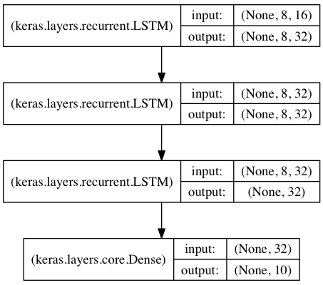
In this model, we stack 3 LSTM layers on top of each other, making the model capable of learning higher-level temporal representations.

The first two LSTMs return their full output sequences, but the last one only returns the last step in its output sequence, thus dropping the temporal dimension (i.e. converting the input sequence into a single vector).

from keras.models import Sequential
from keras.layers import LSTM, Dense
import numpy as np

data_dim = 16
timesteps = 8
nb_classes = 10

# expected input data shape: (batch_size, timesteps, data_dim)
model = Sequential()
model.add(LSTM(32, return_sequences=True,
               input_shape=(timesteps, data_dim)))  # returns a sequence of vectors of dimension 32
model.add(LSTM(32, return_sequences=True))  # returns a sequence of vectors of dimension 32
model.add(LSTM(32))  # return a single vector of dimension 32
model.add(Dense(10, activation='softmax'))

model.compile(loss='categorical_crossentropy',
              optimizer='rmsprop',
              metrics=['accuracy'])

# generate dummy training data
x_train = np.random.random((1000, timesteps, data_dim))
y_train = np.random.random((1000, nb_classes))

# generate dummy validation data
x_val = np.random.random((100, timesteps, data_dim))
y_val = np.random.random((100, nb_classes))

model.fit(x_train, y_train,
          batch_size=64, nb_epoch=5,
          validation_data=(x_val, y_val))

Same stacked LSTM model, rendered "stateful"

A stateful recurrent model is one for which the internal states (memories) obtained after processing a batch of samples are reused as initial states for the samples of the next batch. This allows to process longer sequences while keeping computational complexity manageable.

You can read more about stateful RNNs in the FAQ.

from keras.models import Sequential
from keras.layers import LSTM, Dense
import numpy as np

data_dim = 16
timesteps = 8
nb_classes = 10
batch_size = 32

# expected input batch shape: (batch_size, timesteps, data_dim)
# note that we have to provide the full batch_input_shape since the network is stateful.
# the sample of index i in batch k is the follow-up for the sample i in batch k-1.
model = Sequential()
model.add(LSTM(32, return_sequences=True, stateful=True,
               batch_input_shape=(batch_size, timesteps, data_dim)))
model.add(LSTM(32, return_sequences=True, stateful=True))
model.add(LSTM(32, stateful=True))
model.add(Dense(10, activation='softmax'))

model.compile(loss='categorical_crossentropy',
              optimizer='rmsprop',
              metrics=['accuracy'])

# generate dummy training data
x_train = np.random.random((batch_size * 10, timesteps, data_dim))
y_train = np.random.random((batch_size * 10, nb_classes))

# generate dummy validation data
x_val = np.random.random((batch_size * 3, timesteps, data_dim))
y_val = np.random.random((batch_size * 3, nb_classes))

model.fit(x_train, y_train,
          batch_size=batch_size, nb_epoch=5,
          validation_data=(x_val, y_val))

Two merged LSTM encoders for classification over two parallel sequences

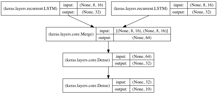
In this model, two input sequences are encoded into vectors by two separate LSTM modules.

These two vectors are then concatenated, and a fully connected network is trained on top of the concatenated representations.

from keras.models import Sequential
from keras.layers import Merge, LSTM, Dense
import numpy as np

data_dim = 16
timesteps = 8
nb_classes = 10

encoder_a = Sequential()
encoder_a.add(LSTM(32, input_shape=(timesteps, data_dim)))

encoder_b = Sequential()
encoder_b.add(LSTM(32, input_shape=(timesteps, data_dim)))

decoder = Sequential()
decoder.add(Merge([encoder_a, encoder_b], mode='concat'))
decoder.add(Dense(32, activation='relu'))
decoder.add(Dense(nb_classes, activation='softmax'))

decoder.compile(loss='categorical_crossentropy',
                optimizer='rmsprop',
                metrics=['accuracy'])

# generate dummy training data
x_train_a = np.random.random((1000, timesteps, data_dim))
x_train_b = np.random.random((1000, timesteps, data_dim))
y_train = np.random.random((1000, nb_classes))

# generate dummy validation data
x_val_a = np.random.random((100, timesteps, data_dim))
x_val_b = np.random.random((100, timesteps, data_dim))
y_val = np.random.random((100, nb_classes))

decoder.fit([x_train_a, x_train_b], y_train,
            batch_size=64, nb_epoch=5,
            validation_data=([x_val_a, x_val_b], y_val))